The code of these examples can be found in the examples package. The first three examples are meant to illustrate the basics of the EMA workbench. How to implement a model, specify its uncertainties and outcomes, and run it. The fourth example is a more extensive illustration based on Pruyt & Hamarat (2010). It shows some more advanced possibilities of the EMA workbench, including one way of handling policies.
In order to perfom EMA on a model. The first step is to extent ModelStructureInterface.
1 2 3 4 5 6 | class SimplePythonModel(ModelStructureInterface):
'''
This class represents a simple example of how one can extent the basic
ModelStructureInterface in order to do EMA on a simple model coded in
Python directly
'''
|
we need to specify the uncertainties and outcomes and implement at least two methods :
- model_init()
- run_model()
We can specify the uncertainties and outcomes directly by assiging them to self.uncertainties and self.outcomes respectively, Below, we specify three ParameterUncertainty instances, with the names ‘x1’, ‘x2’, and ‘x3’, and add them to self.uncertainties. The first argument when instantiating ParameterUncertainty specifies the range over which we want to sample. So, the value of ‘x1’ is defined as being somewhere between 0.1 and 10. Then, we have to specify the outcomes that the model generates. In this example we have only a single Outcome instance, called ‘y’.
1 2 3 4 5 6 7 | #specify uncertainties
uncertainties = [ParameterUncertainty((0.1, 10), "x1"),
ParameterUncertainty((-0.01,0.01), "x2"),
ParameterUncertainty((-0.01,0.01), "x3")]
#specify outcomes
outcomes = [Outcome('y')]
|
Having specified the uncertainties ant the outcomes, we can now implement model_init(). Since this is a simple example, we can suffice with a ‘pass’. Meaning we do not do anything. In case of more complex models, model_init() can be used for setting policy related variables, and/or starting external tools or programs(e.g. Java, Excel, Vensim).
def model_init(self, policy, kwargs):
pass
Finally, we implement run_model(). Here we have a very simple model:
def run_model(self, case):
"""Method for running an instantiated model structure """
self.output[self.outcomes[0].name] = case['x1']*case['x2']+case['x3']
The above code might seem a bit strange. There are a couple of things being done in a single line of code. First, we need to assign the outcome to self.output, which should be a dict. The key should match the names of the outcomes as specified in self.outcomes. Since we have only 1 outcome, we can get to its name directly.
self.outcomes[0].name #this gives us the name of the first entry in self.outcomes
Next, we assign as value the outcome of our model. Here case[‘x1’] gives us
the value of ‘x1’. So our model is  . Which in python code
with the values for ‘x1’, ‘x2’, and ‘x3’ stored in the case dict looks like
the following:
. Which in python code
with the values for ‘x1’, ‘x2’, and ‘x3’ stored in the case dict looks like
the following:
case['x1']*case['x2']+case['x3'] #this gives us the outcome
Having implemented this model, we can now do EMA by executing the following code snippet
1 2 3 4 5 6 | from expWorkbench import ModelEnsemble
model = SimplePythonModel(None, 'simpleModel') #instantiate the model
ensemble = ModelEnsemble() #instantiate an ensemble
ensemble.set_model_structure(model) #set the model on the ensemble
results = ensemble.perform_experiments(1000) #generate 1000 cases
|
Here, we instantiate the model first. Instantiating a model requires two arguments: a working directory, and a name. The latter is required, the first is not. Our model does not have a working directory, so we pass None. Next we instantiate a ModelEnsemble and add the model to it. This class handles the generation of the experimetns, the executing of the experiments, and the storing of the results. We perform the experiments by invoing the perform_experiments().
The complete code:
1 2 3 4 5 6 7 8 9 10 11 12 13 14 15 16 17 18 19 20 21 22 23 24 25 26 27 28 29 30 31 32 33 34 35 36 37 38 39 | '''
Created on 20 dec. 2010
This file illustrated the use the EMA classes for a contrived example
It's main purpose has been to test the parallel processing functionality
.. codeauthor:: jhkwakkel <j.h.kwakkel (at) tudelft (dot) nl>
'''
from expWorkbench import ModelEnsemble, ModelStructureInterface,\
ParameterUncertainty, Outcome
class SimplePythonModel(ModelStructureInterface):
    '''
    This class represents a simple example of how one can extent the basic
    ModelStructureInterface in order to do EMA on a simple model coded in
    Python directly
    '''
#specify uncertainties
uncertainties = [ParameterUncertainty((0.1, 10), "x1"),
ParameterUncertainty((-0.01,0.01), "x2"),
ParameterUncertainty((-0.01,0.01), "x3")]
#specify outcomes
outcomes = [Outcome('y')]
def model_init(self, policy, kwargs):
pass
def run_model(self, case):
"""Method for running an instantiated model structure """
self.output[self.outcomes[0].name] = case['x1']*case['x2']+case['x3']
if __name__ == '__main__':
model = SimplePythonModel(None, 'simpleModel') #instantiate the model
ensemble = ModelEnsemble() #instantiate an ensemble
ensemble.set_model_structure(model) #set the model on the ensemble
results = ensemble.perform_experiments(1000) #generate 1000 cases
|
In order to perfom EMA on a model build in Vensim, we can either extent ModelStructureInterface or use VensimModelStructureInterface. The later contains a boiler plate implementation for starting vensim, setting parameters, running the model, and retrieving the results. VensimModelStructureInterface is thus the most obvious choice. For almost all cases when performing EMA on Vensim model, VensimModelStructureInterface can serve as the base class.
Imagine we have a very simple Vensim model:
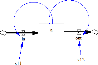
For this example, we assume that ‘x11’ and ‘x12’ are uncertain. The state variable ‘a’ is the outcome of interest. We are going to extent VensimModelStructureInterface accordingly.
1 2 3 4 5 6 7 8 9 10 11 12 13 14 15 16 17 | class VensimExampleModel(VensimModelStructureInterface):
'''
example of the most simple case of doing EMA on
a vensim model
'''
#note that this reference to the model should be relative
#this relative path will be combined to the workingDirectory
modelFile = r'\model.vpm'
#specify outcomes
outcomes = [Outcome('a', time=True)]
#specify your uncertainties
uncertainties = [ParameterUncertainty((0, 2.5), "x11"),
ParameterUncertainty((-2.5, 2.5), "x12")]
|
We make a class called VensimExampleModel that extents VensimModelStructureInterface. For the simplest case, we only need to specify the model file, the outcomes, and the uncertainties.
We specify the model file relative to the working directory.
modelFile = r'\model.vpm'
We add an Outcome called ‘a’ to self.outcomes. The second argument time=True means we are interested in the value of ‘a’ over the duration of the simulation.
outcomes = [Outcome('a', time=True)]
We add two ParameterUncertainty instances titled ‘x11’ and ‘x12’ to self.uncertainties.
uncertainties = [ParameterUncertainty((0, 2.5), "x11"),
ParameterUncertainty((-2.5, 2.5), "x12")]
By specifying these three elements -the path to the model file relative to a working directory, the outcomes, and the uncertainties- we are now able to perform EMA on the simple Vensim model.
1 2 3 4 5 6 7 8 9 10 11 12 13 14 15 16 17 | #turn on logging
ema_logging.log_to_stderr(ema_logging.INFO)
#instantiate a model
vensimModel = VensimExampleModel(r"..\..\models\vensim example", "simpleModel")
#instantiate an ensemble
ensemble = ModelEnsemble()
#set the model on the ensemble
ensemble.set_model_structure(vensimModel)
#run in parallel, if not set, FALSE is assumed
ensemble.parallel = True
#perform experiments
result = ensemble.perform_experiments(1000)
|
In the first line, we turn on the logging functionality provided by ema_logging. This is highly recommended, for we can get much more insight into what is going on: how the simulations are progressing, whether there are any warnings or errors, etc. For normal runs, we can set the level to the INFO level, which in most cases is sufficient. For more details see ema_logging.
The complete code
1 2 3 4 5 6 7 8 9 10 11 12 13 14 15 16 17 18 19 20 21 22 23 24 25 26 27 28 29 30 31 32 33 34 35 36 37 38 39 40 41 42 43 44 45 46 47 48 49 | '''
Created on 3 Jan. 2011
This file illustrated the use the EMA classes for a contrived example
It's main purpose is to test the parallel processing functionality
.. codeauthor:: jhkwakkel <j.h.kwakkel (at) tudelft (dot) nl>
chamarat <c.hamarat (at) tudelft (dot) nl>
'''
from expWorkbench import ModelEnsemble, ParameterUncertainty, Outcome,\
ema_logging
from expWorkbench.vensim import VensimModelStructureInterface
class VensimExampleModel(VensimModelStructureInterface):
'''
example of the most simple case of doing EMA on
a Vensim model.
'''
#note that this reference to the model should be relative
#this relative path will be combined with the workingDirectory
modelFile = r'\model.vpm'
#specify outcomes
outcomes = [Outcome('a', time=True)]
#specify your uncertainties
uncertainties = [ParameterUncertainty((0, 2.5), "x11"),
ParameterUncertainty((-2.5, 2.5), "x12")]
if __name__ == "__main__":
#turn on logging
ema_logging.log_to_stderr(ema_logging.INFO)
#instantiate a model
vensimModel = VensimExampleModel(r"..\..\models\vensim example", "simpleModel")
#instantiate an ensemble
ensemble = ModelEnsemble()
#set the model on the ensemble
ensemble.set_model_structure(vensimModel)
#run in parallel, if not set, FALSE is assumed
ensemble.parallel = True
#perform experiments
result = ensemble.perform_experiments(1000)
|
In order to perform EMA on an Excel model, the easiest is to use ExcelModelStructureInterface as the base class. This base class makes uses of naming cells in Excell to refer to them directly. That is, we can assume that the names of the uncertainties correspond to named cells in Excell, and similarly, that the names of the outcomes correspond to named cells or ranges of cells in Excel. When using this class, make sure that the decimal seperator and thousands seperator are set correctly in Excel. This can be checked via file > options > advanced. These seperators should follow the anglo saxon convention.
1 2 3 4 5 6 7 8 9 10 11 12 13 14 15 16 17 18 19 20 21 22 23 24 25 26 27 28 29 30 31 32 33 34 35 36 37 38 39 40 41 42 43 44 45 46 47 48 49 50 51 52 53 54 55 56 57 58 59 60 61 62 63 64 | '''
Created on 27 Jul. 2011
This file illustrated the use the EMA classes for a model in Excel.
It used the excel file provided by
`A. Sharov <http://home.comcast.net/~sharov/PopEcol/lec10/fullmod.html>`_
This excel file implements a simple predator prey model.
.. codeauthor:: jhkwakkel <j.h.kwakkel (at) tudelft (dot) nl>
'''
import matplotlib.pyplot as plt
from expWorkbench import ModelEnsemble, ParameterUncertainty,\
Outcome, ema_logging
from expWorkbench.excel import ExcelModelStructureInterface
from analysis.plotting import lines
class ExcelModel(ExcelModelStructureInterface):
uncertainties = [ParameterUncertainty((0.01, 0.2),
"K2"), #we can refer to a cell in the normal way
ParameterUncertainty((450,550),
"KKK"), # we can also use named cells
ParameterUncertainty((0.05,0.15),
"rP"),
ParameterUncertainty((0.00001,0.25),
"aaa"),
ParameterUncertainty((0.45,0.55),
"tH"),
ParameterUncertainty((0.1,0.3),
"kk")]
#specification of the outcomes
outcomes = [Outcome("B4:B1076", time=True), #we can refer to a range in the normal way
Outcome("P_t", time=True)] # we can also use named range
#name of the sheet
sheet = "Sheet1"
#relative path to the Excel file
workbook = r'\excel example.xlsx'
if __name__ == "__main__":
logger = ema_logging.log_to_stderr(level=ema_logging.INFO)
model = ExcelModel(r"..\..\models\excelModel", "predatorPrey")
ensemble = ModelEnsemble()
ensemble.set_model_structure(model)
ensemble.parallel = True #turn on parallel computing
ensemble.processes = 2 #using only 2 cores
#generate 100 cases
results = ensemble.perform_experiments(10)
lines(results)
plt.show()
#save results
# save_results(results, r'..\..\excel runs.cPickle')
|
The example is relatively straight forward. We add multiple ParameterUncertainty instances to self.uncertainties. Next, we add two outcome to self.outcomes. We specify the name of the sheet (self.sheet) and the relative path to the workbook (self.workbook). This compleets the specification of the Excel model.
Warning
when using named cells. Make sure that the names are defined at the sheet level and not at the workbook level!
This example is derived from Pruyt & Hamarat (2010). This paper presents a small exploratory System Dynamics model related to the dynamics of the 2009 flu pandemic, also known as the Mexican flu, swine flu, or A(H1N1)v. The model was developed in May 2009 in order to quickly foster understanding about the possible dynamics of this new flu variant and to perform rough-cut policy explorations. Later, the model was also used to further develop and illustrate Exploratory Modelling and Analysis.
In the first days, weeks and months after the first reports about the outbreak of a new flu variant in Mexico and the USA, much remained unknown about the possible dynamics and consequences of the at the time plausible/imminent epidemic/pandemic of the new flu variant, first known as Swine or Mexican flu and known today as Influenza A(H1N1)v.
The exploratory model presented here is small, simple, high-level, data-poor (no complex/special structures nor detailed data beyond crude guestimates), and history-poor.
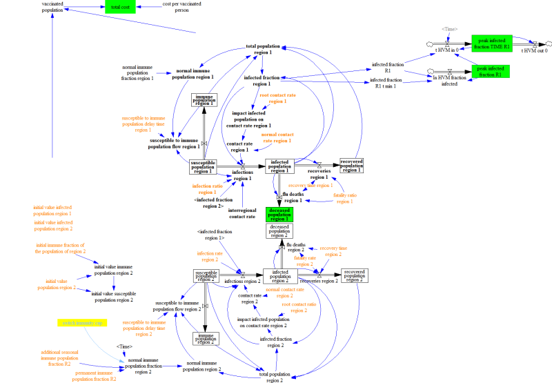
The modelled world is divided in three regions: the Western World, the densely populated Developing World, and the scarcely populated Developing World. Only the two first regions are included in the model because it is assumed that the scarcely populated regions are causally less important for dynamics of flu pandemics. Below, the figure shows the basic stock-and-flow structure. For a more elaborate description of the model, see Pruyt & Hamarat (2010).
Given the various uncertainties about the exact characteristics of the flu, including its fatality rate, the contact rate, the susceptability of the population, etc. the flu case is an ideal candiate for EMA. One can use EMA to explore the kinds of dynamics that can occur, identify undesirable dynamic, and develop policies targeted at the undesirable dynamics.
In the orignal paper, Pruyt & Hamarat (2010). recoded the model in Python and performed the analysis in that way. Here we show how the EMA workbench can be connected to Vensim directly.
The flu model was build in Vensim. We can thus use VensimModelStructureInterface as a base class.
We are interessted in two outcomes:
- deceased population region 1: the total number of deaths over the duration of the simulation.
- peak infected fraction: the fraction of the population that is infected.
These are added to self.outcomes. time is set to True, meaning we want their values over the entire run.
The table below is adapted from Pruyt & Hamarat (2010). It shows the uncertainties, and their bounds. These are added to self.uncertainties as ParameterUncertainty instances.
| Parameter | Lower Limit | Upper Limit |
|---|---|---|
| additional seasonal immune population fraction region 1 | 0.0 | 0.5 |
| additional seasonal immune population fraction region 2 | 0.0 | 0.5 |
| fatality ratio region 1 | 0.0001 | 0.1 |
| fatality ratio region 2 | 0.0001 | 0.1 |
| initial immune fraction of the population of region 1 | 0.0 | 0.5 |
| initial immune fraction of the population of region 2 | 0.0 | 0.5 |
| normal interregional contact rate | 0.0 | 0.9 |
| permanent immune population fraction region 1 | 0.0 | 0.5 |
| permanent immune population fraction region 2 | 0.0 | 0.5 |
| recovery time region 1 | 0.2 | 0.8 |
| recovery time region 2 | 0.2 | 0.8 |
| root contact rate region 1 | 1.0 | 10.0 |
| root contact rate region 2 | 1.0 | 10.0 |
| infection ratio region 1 | 0.0 | 0.1 |
| infection ratio region 2 | 0.0 | 0.1 |
| normal contact rate region 1 | 10 | 200 |
| normal contact rate region 2 | 10 | 200 |
Together, this results in the following code:
1 2 3 4 5 6 7 8 9 10 11 12 13 14 15 16 17 18 19 20 21 22 23 24 25 26 27 28 29 30 31 32 33 34 35 36 37 38 39 40 41 42 43 44 45 46 47 48 49 50 51 52 53 54 55 56 57 58 59 60 61 62 63 64 65 66 67 68 69 70 71 72 73 74 75 76 77 | '''
Created on 20 May, 2011
This module shows how you can use vensim models directly
instead of coding the model in Python. The underlying case
is the same as used in fluExample
.. codeauthor:: jhkwakkel <j.h.kwakkel (at) tudelft (dot) nl>
epruyt <e.pruyt (at) tudelft (dot) nl>
'''
from expWorkbench import ModelEnsemble, ParameterUncertainty,\
Outcome, save_results, ema_logging
from expWorkbench.vensim import VensimModelStructureInterface
class FluModel(VensimModelStructureInterface):
#base case model
modelFile = r'\FLUvensimV1basecase.vpm'
#outcomes
outcomes = [Outcome('deceased population region 1', time=True),
Outcome('infected fraction R1', time=True)]
#Plain Parametric Uncertainties
uncertainties = [
ParameterUncertainty((0, 0.5),
"additional seasonal immune population fraction R1"),
ParameterUncertainty((0, 0.5),
"additional seasonal immune population fraction R2"),
ParameterUncertainty((0.0001, 0.1),
"fatality ratio region 1"),
ParameterUncertainty((0.0001, 0.1),
"fatality rate region 2"),
ParameterUncertainty((0, 0.5),
"initial immune fraction of the population of region 1"),
ParameterUncertainty((0, 0.5),
"initial immune fraction of the population of region 2"),
ParameterUncertainty((0, 0.9),
"normal interregional contact rate"),
ParameterUncertainty((0, 0.5),
"permanent immune population fraction R1"),
ParameterUncertainty((0, 0.5),
"permanent immune population fraction R2"),
ParameterUncertainty((0.1, 0.75),
"recovery time region 1"),
ParameterUncertainty((0.1, 0.75),
"recovery time region 2"),
ParameterUncertainty((0.5,2),
"susceptible to immune population delay time region 1"),
ParameterUncertainty((0.5,2),
"susceptible to immune population delay time region 2"),
ParameterUncertainty((0.01, 5),
"root contact rate region 1"),
ParameterUncertainty((0.01, 5),
"root contact ratio region 2"),
ParameterUncertainty((0, 0.15),
"infection ratio region 1"),
ParameterUncertainty((0, 0.15),
"infection rate region 2"),
ParameterUncertainty((10, 100),
"normal contact rate region 1"),
ParameterUncertainty((10, 200),
"normal contact rate region 2")]
if __name__ == "__main__":
ema_logging.log_to_stderr(ema_logging.INFO)
model = FluModel(r'..\..\models\flu', "fluCase")
ensemble = ModelEnsemble()
ensemble.set_model_structure(model)
ensemble.parallel = True #turn on parallel processing
results = ensemble.perform_experiments(1000)
save_results(results, r'1000 flu cases no policy.bz2')
|
We can now instantiate the model, instantiate an ensemble, and set the model on the ensemble, as seen below. Just as witht the simple Vensim model, we first start the logging and direct it to the stream specified in sys.stderr. Which, if we are working with Eclipse is the console. Assuming we have imported ModelEnsemble and ema_logging, we can do the following
1 2 3 4 5 6 7 8 9 | EMALogging.log_to_stderr(level=EMALogging.INFO)
model = FluModel(r'..\..\models\flu', "fluCase")
ensemble = ModelEnsemble()
ensemble.set_model_structure(model)
ensemble.parallel = True
results = ensemble.perform_experiments(1000)
|
We now have generated a 1000 cases and can proceed to analyse the results using various analysis scripts. As a first step, one can look at the individual runs using a line plot using lines(). See plotting for some more visualizations using results from performing EMA on FluModel.
1 2 3 4 5 | import matplotlib.pyplot as plt
from analysis.plotting import lines
figure = lines(results, density=True) #show lines, and end state density
plt.show() #show figure
|
generates the following figure:
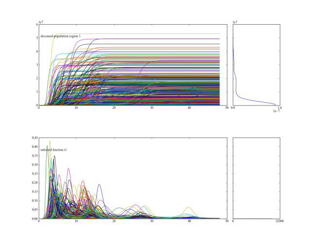
From this figure, one can deduce that accross the ensemble of possible futures, there is a subset of runs with a substantial ammount of deaths. We can zoom in on those cases, identify their conditions for occuring, and use this insight for policy design.
For further analysis, it is generally conveniened, to generate the results for a series of experiments and save these results. One can then use these saved results in various analysis scripts.
from expWorkbench.util import save_results
save_results(results, model.workingDirectory+r'\1000 runs.bz2')
The above code snippet shows how we can use save_results() for saving the results of our experiments. save_results() stores the results using cPickle and bz2. It is recommended to use save_results(), instead of using cPickle directly, to guarantee cross-platform useability of the stored results. That is, one can generate the results on say Windows, but still open them on say MacOs. The extensions .bz2 is strictly speaking not necessary, any file extension can be used, but it is found convenient to easily identify saved results.
For this paper, policies were developed by using the system understanding of the analysts.
In order to be able to run the models with the policies and to compare their results with the no policy case, we need to modify FluModel. We overide the default implementation of model_init() to change the model file based on the policy. After this, we call the super.
1 2 3 4 5 6 7 8 | def model_init(self, policy, kwargs):
'''initializes the model'''
try:
self.modelFile = policy['file']
except KeyError:
logging.warning("key 'file' not found in policy")
super(FluModel, self).model_init(policy, kwargs)
|
Now, our model can react to different policies, but we still have to add these policies to ModelEnsemble. We therefore make a list of policies. Each entry in the list is a dict, with a ‘name’ field and a ‘file’ field. The name specifies the name of the policy, and the file specified the model file to be used. We add this list of policies to the ensemble.
1 2 3 4 5 6 7 8 9 | #add policies
policies = [{'name': 'no policy',
'file': r'\FLUvensimV1basecase.vpm'},
{'name': 'static policy',
'file': r'\FLUvensimV1static.vpm'},
{'name': 'adaptive policy',
'file': r'\FLUvensimV1dynamic.vpm'}
]
ensemble.add_policies(policies)
|
We can now proceed in the same way as before, and perform a series of experiments. Together, this results in the following code:
1 2 3 4 5 6 7 8 9 10 11 12 13 14 15 16 17 18 19 20 21 22 23 24 25 26 27 28 29 30 31 32 33 34 35 36 37 38 39 40 41 42 43 44 45 46 47 48 49 50 51 52 53 54 55 56 57 58 59 60 61 62 63 64 65 66 67 68 69 70 71 72 73 74 75 76 77 78 79 80 81 82 83 84 85 86 87 88 89 90 91 92 93 94 95 | '''
Created on 20 May, 2011
This module shows how you can use vensim models directly
instead of coding the model in Python. The underlying case
is the same as used in fluExample
.. codeauthor:: jhkwakkel <j.h.kwakkel (at) tudelft (dot) nl>
epruyt <e.pruyt (at) tudelft (dot) nl>
'''
from expWorkbench import ModelEnsemble, ParameterUncertainty,\
Outcome, save_results, ema_logging
from expWorkbench.vensim import VensimModelStructureInterface
class FluModel(VensimModelStructureInterface):
#base case model
modelFile = r'\FLUvensimV1basecase.vpm'
#outcomes
outcomes = [Outcome('deceased population region 1', time=True),
Outcome('infected fraction R1', time=True)]
#Plain Parametric Uncertainties
uncertainties = [
ParameterUncertainty((0, 0.5),
"additional seasonal immune population fraction R1"),
ParameterUncertainty((0, 0.5),
"additional seasonal immune population fraction R2"),
ParameterUncertainty((0.0001, 0.1),
"fatality ratio region 1"),
ParameterUncertainty((0.0001, 0.1),
"fatality rate region 2"),
ParameterUncertainty((0, 0.5),
"initial immune fraction of the population of region 1"),
ParameterUncertainty((0, 0.5),
"initial immune fraction of the population of region 2"),
ParameterUncertainty((0, 0.9),
"normal interregional contact rate"),
ParameterUncertainty((0, 0.5),
"permanent immune population fraction R1"),
ParameterUncertainty((0, 0.5),
"permanent immune population fraction R2"),
ParameterUncertainty((0.1, 0.75),
"recovery time region 1"),
ParameterUncertainty((0.1, 0.75),
"recovery time region 2"),
ParameterUncertainty((0.5,2),
"susceptible to immune population delay time region 1"),
ParameterUncertainty((0.5,2),
"susceptible to immune population delay time region 2"),
ParameterUncertainty((0.01, 5),
"root contact rate region 1"),
ParameterUncertainty((0.01, 5),
"root contact ratio region 2"),
ParameterUncertainty((0, 0.15),
"infection ratio region 1"),
ParameterUncertainty((0, 0.15),
"infection rate region 2"),
ParameterUncertainty((10, 100),
"normal contact rate region 1"),
ParameterUncertainty((10, 200),
"normal contact rate region 2")]
def model_init(self, policy, kwargs):
'''initializes the model'''
try:
self.modelFile = policy['file']
except KeyError:
ema_logging.warning("key 'file' not found in policy")
super(FluModel, self).model_init(policy, kwargs)
if __name__ == "__main__":
ema_logging.log_to_stderr(ema_logging.INFO)
model = FluModel(r'..\..\models\flu', "fluCase")
ensemble = ModelEnsemble()
ensemble.set_model_structure(model)
#add policies
policies = [{'name': 'no policy',
'file': r'\FLUvensimV1basecase.vpm'},
{'name': 'static policy',
'file': r'\FLUvensimV1static.vpm'},
{'name': 'adaptive policy',
'file': r'\FLUvensimV1dynamic.vpm'}
]
ensemble.add_policies(policies)
ensemble.parallel = True #turn on parallel processing
results = ensemble.perform_experiments(1000)
save_results(results, r'./data/1000 flu cases.bz2')
|
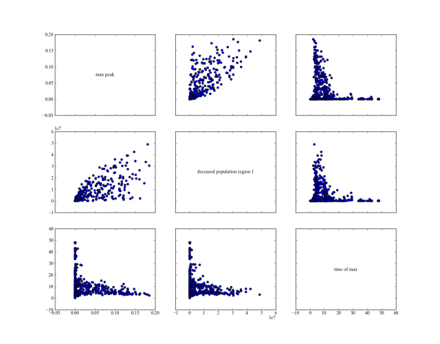
Using the following script, we reproduce figures similar to the 3D figures in Pruyt & Hamarat (2010). But using pairs_scatter(). It shows for the three different policies their behavior on the total number of deaths, the hight of the heighest peak of the pandemic, and the point in time at which this peak was reached.
1 2 3 4 5 6 7 8 9 10 11 12 13 14 15 16 17 18 19 20 21 22 23 24 25 26 27 28 29 30 31 32 33 34 35 36 37 38 39 40 | '''
Created on 20 sep. 2011
.. codeauthor:: jhkwakkel <j.h.kwakkel (at) tudelft (dot) nl>
'''
import numpy as np
import matplotlib.pyplot as plt
from analysis.pairs_plotting import pairs_lines, pairs_scatter, pairs_density
from expWorkbench.util import load_results
from expWorkbench import ema_logging
ema_logging.log_to_stderr(level=ema_logging.DEFAULT_LEVEL)
#load the data
experiments, outcomes = load_results(r'.\data\100 flu cases no policy.bz2')
#transform the results to the required format
newResults = {}
#get time and remove it from the dict
time = outcomes.pop('TIME')
for key, value in outcomes.items():
if key == 'deceased population region 1':
newResults[key] = value[:,-1] #we want the end value
else:
# we want the maximum value of the peak
newResults['max peak'] = np.max(value, axis=1)
# we want the time at which the maximum occurred
# the code here is a bit obscure, I don't know why the transpose
# of value is needed. This however does produce the appropriate results
logicalIndex = value.T==np.max(value, axis=1)
newResults['time of max'] = time[logicalIndex.T]
pairs_scatter((experiments, newResults))
pairs_lines((experiments, newResults))
pairs_density((experiments, newResults))
plt.show()
|
no policy
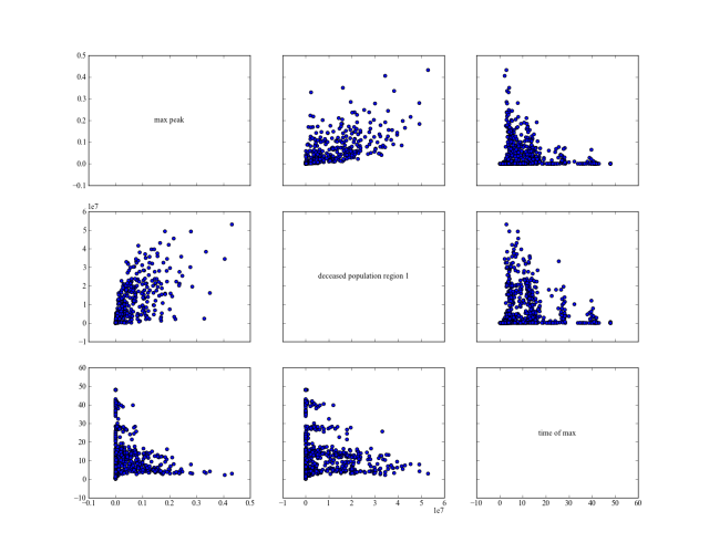
static policy
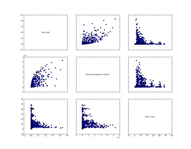
adaptive policy